Closed-loop Controls
PID
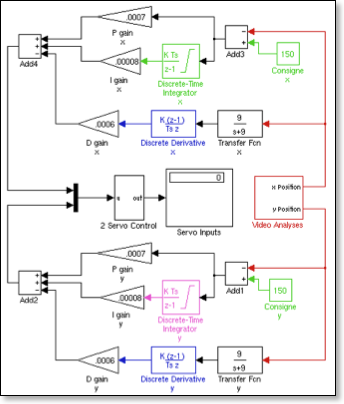
Proportional: The difference between where you are and where you want to be is called the error, which we then multiply by some constant. For example, if you were 2cm from your target, the P control value would be twice as big as if you were 1cm away. Thus, the further you are away from your set-point, the more control input you have.
Integral: The above error is integrated over time and multiplied by a second constant, that is to say that for each second where you are still not at your set-point, the I control value gets bigger and bigger. This integrator smoothes out inconsistencies in the model by slowly but surely modifying the control value. Take the example of the table. If my table weren't perfectly flat, which is the case, and it were sitting on a surface that weren't perfectly level, again the case, then all my calculations would amount to nothing, as the ball could never get to its destination because of these imperfections. However, the integrator slowly (or quickly depending on how big the constant is,) adjusts so that it's level.
Derivative: The derivative of the observed variable is taken, that is to say we divide its change by the time. Tn the case of my ball, this gives us its speed, and allows us to dampen the movement. The derivative is multiplied by a third constant for the D control. The higher the constant, the more the table tries to slow down the movement of the ball. This is very useful in getting the ball to stop rapidly.
In a perfect world, you would have a high P constant (to arrive very quickly at the destination), a high D constant (to stop quickly at the destination without overshooting), and a low I constant (if the system is good, you won't need much integration in order to overcome basic imperfections.
I used a PID as a first controller because it's quite good and very easy to make. In fact, a PID can be made inside of 5 minutes, although it takes a little longer to get it fine-tuned.
However, the PID is a temporary solution, handy because it's easy, but not very intelligent because it has no knowledge of the model. Thus, as a first step it's acceptable, but we can do better.
For a more rigorous explanation, click here.
LQR Controller
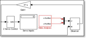
LQR controllers offer the opportunity to weight various values in the state vector, for instance valuing more the speed than the position of the ball as it rolls. In effect, this means that the controller will place less emphasis on being in the correct spot and more emphasis on stabilizing the speed. Furthermore, the controller can be adjusted to react more vehemently, if it's more important that the system be controlled than, say, saving the equipment by not moving too brusquely.
I use an LQR for much of what I do as it's a good all around controller. I also improve it's performance by coupling it with an integrator part from a PID in order to smooth out imperfections in my model and finally arrive at the correct target.
For a more rigorous explanation, click here.
Geometric control
Geometric control is a very interesting controls scheme that requires a very good correlation between the real and the theoretic models. In geometric control, we decide in advance how we want the system to go from one state to another. For instance, we decide that ideally, the ball should start off stopped and the table level, the ball should then accelerate smoothly, roll a distance, and then decelerate smoothly before stopping at the end of a once-again level table. All this in a prescribe time, for example 3 seconds.
So, in an perfect world, the ball will exactly follow this family of curves. Even if it goes too fast or too slow, leaving the ideal curve, it will simply join another curve in the family that will still bring it to the end. However, this can prove very problematic at the end as when the ball is almost upon the target, the table tends to get rushed, and starts giving large commands in order to reach the set-point at the intended time.
We can illustrate this with my above example of three seconds from start to finish. When the controller is in the first second of the maneuver, it still has plenty of time so only small modifications are necessary. Whereas, once the ball is almost there, if it's a little too close or a little too far the table has to react very violently in order to ensure that the ball arrives at the destination at precisely 3.0000 seconds.
This is a problem with geometric control, but the solution is easy enough. I developed a controller that uses both PID and geometric controllers. At the beginning, the PID has no effect whatsoever, but as the ball gets closer and closer to the target the PID's influence becomes greater and greater. Thus, at 90% of the distance, the PID is in almost complete control, thus eliminating the geometric controller's oversensitivity to noise in the last moments of the control.
For a more rigorous explanation, click here.