• Introduction
• Construction and Design
• Mathematical Theory and Application
• Simulacrum and Simulation
• Conclusion and Current State of the Art
• Appendix
  • Pea and Spoon Effect
  • Automatic Dial Reader
  • Camera Calibration Code
  • Observer and Observability
  • Controller and Controllability

• Introduction > 
• Appendix > 
• Controller and Controllability > 

Controller and Controllability

Controllability

A system is said to be controllable if for all vector pairs (x_d, x_a) in Rⁿ there exists a finite time T and a command u defined on [0,T] such that when the command u is applied the solution x(t) starting from x(0)=x_d gives x(T)=x_a.

In layman’s terms, a system is controllable if you can start at A and apply commands to finish at B. Obvious, eh?
Mathematically speaking, the system is controllable iff the controllability matrix



is rank n.

PID controller

Every system has a transfer function (even if we don't know it and can't write it down) whereby an input u has an output y. The PID is a transfer function that places the roots of the system’s transfer function/PID function in a stable location, i.e. the real part of the roots is negative.

Mathematically:



is the closed-loop system’s transfer function, where V is the Laplace transform of the external stimulus, H is the system, Y is the output, and G(s) is the PID.



By choosing K_p, K_d, and K_i, you’re placing the roots of the closed-loop transfer function strictly to the right of the y-axis. These roots can be chosen mathematically in advance, if you have some knowledge of the system, or empirically after-the-fact.
For even more on PIDs, the ball and beam, and Matlab, click here.

LQR controller

An LQR controller seeks to minimize the quadratic equation:



by using the Riccati equations:



Which gives the ideal control u=-K*x with:



Where Q and R are the relative weights of the cost of the control, and N is usually [0].

The lower R is, the more it costs to get to the destination but the faster you get there, and vice-versa. The individual elements of Q are weighted, meaning that we can place a higher priority on one variable, for instance, due to the geometry of my table, when I turn in two servo mode I get better performance when Q=[10 0 0 0; 0 1 0 0; 0 0 10 0; 0 0 0 1]. In this example, R=1 gives a quite good response rate that's not so fast that the table shakes itself apart but not so slow that the controller takes forever and a day to steer the ball to its destination.

For a better explanation of how the LQR controller works on the ball and beam system, click here.

For an explanation of the Matlab function, click here.

Geometric controller

The geometric controller is a much more complicated, much more idealistic controller than the other two above. It's advantage, however, is that we get to define the ball's behavior in a very strict sense.

First we define a ball trajectory. In this case, we specified that the ball must be motionless at the beginning, motionless at the end, and must have null acceleration at the end (i.e. the table is flat).

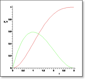
This gives us a position vs. time trajectory and a velocity vs. time trajectory. In the graph at right, the red curve is the position, the green curve the velocity, the x-axis is time, and the y-axis is in meters.

Once we have these trajectories, we can plot the behavior of the table to ensure that the table doesn't have to react too quickly in order to follow our curves

We can see this in the graph at left. The table starts off at a severe inclination, but mellows out and at the end finishes perfectly at 0.

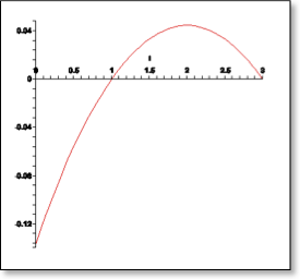
The x-axis is time and the y-axis is deplacement of the pushrod, which direcly correlates with the table's tilt angle.

Finally, this gives us a family of curves that the ball will try to follow. If the ball overshoots one curve, it will still fall on another one. It will simply follow the new curve, instead of trying to catch up to the old one.

• Introduction > 
• Appendix > 
• Controller and Controllability >