Recreating the state vector
As mentioned before, that ball and plate system is observable, and due to controllability reasons, I need to get the ball’s velocity along with its coordinates.
In my case, the most basic way to calculate velocity would be to take the position information and deriving it by time. In other words, I take the position at time A, the position at time B, and divide it by the difference between time A and time B. Voila, a first estimation of velocity.
While this is easy to do and very quick, it's not very good when in noisy environments. For instance, if the ball is stopped, but due to signal noise the computer believes that it just moved by one pixel to the right and then hopped back one pixel to the left, it's going to record that as a very high velocity and an incredibly high acceleration. This is not good, as the table is going to severely spasm trying to stabilize this perceived velocity. I need a better way. This better way is called an observer.
An observer is a mathematical construct that uses physical properties of the system to guess at what all the other properties must be. Well, guess isn't really a good word, as observers are far better than that.
An observer takes the previous state and plugs it into the physical model to get an estimation of where the next state should be, everything being perfect. If everything is perfect, and the model is good, the predicted state and the observed state will be the same. However, more often than not, there are slight-- and sometimes not so slight-- deviations from the model. When the prediction and the observation are not the same, the observer applies a weight to this difference and feeds the weighted results back into the model, outputting a best guess of what the state really is.
While there are many observers available, one of the best and most frequently used is the Kalman Filter. The Kalman filter uses stochastic analysis to create a weight that both allows for rapid convergence to the real solution (if the estimated solution is not the correct one) and allows for noise rejection.
It works in basically the same way as I explained above-- it's magic lies in the way it weights the values and the way that we can decide which values to believe and which values to be wary of. For instance, if for some reason I can measure very precisely movement in the x-direction, but my y-direction measurements aren't so good, I can “inform” the model of this, telling it to place higher confidence on my x-measurements. Furthermore, I can tell the Kalman Filter whether it should globally place a higher priority on the measurements or a higher priority on the model estimations.
As I said, the Kalman Filter observer is also quite well adapted to rejecting noise. For instance, we know that cars are limited in speed, so if I were tracking a car by GPS, and one second I saw the car in Luxembourg and the next second in Italy and the third second back in Luxembourg, I might be inclined to totally reject the data point in Italy as noise.
Equivalently, the observer has knowledge of the table's state and the physics of the ball, so if it finds that the table is tilted to the right, and that for one data point the ball is accelerating to the left, than it simply rejects that data point.
Ball and Plate Observer
The ball and plate system can be described explicitly in a continuous setting.

It so happens that it can also be explicitly written in the discrete time-frame.

where

In the three actuator version, this is a happy coincidence because it means that if I choose a Kalman fliter, our observer can be exact. We do not need to approximate our system, by linearizing it around a stability point for example. Meaning that we simply cannot do better... Of course, if my physical models are incorrect, than of course the observer all this is for naught. However, my Kalman filter ends up being a very, very, very long equation. Too long to put in this paper. In fact, it’s so long, it causes Matlab’s text editor fits.
For simplicity’s sake, and because the estimation is 98.9% correct in the worst of foreseeable cases, we linearized the discrete time-frame equations using the Euler method. This makes for a matrix that is much easier and faster to compute.
However, one caveat is that the previously mentioned observation matrix, C, is in fact in need of correction. Because the camera is not directly over the ball at all times, the projected image is not in the same location as the ball. This is due to perspective and is very easy to solve.
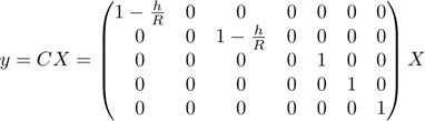
NOTE: This equation assumes that the camera is located at (0,0). If this is not the case, than the measured inputs for x and y need to be shifted so that the origin of the observer coordinate system is at the point directly below the camera. In fact, neglecting this introduces only a small error, on the order of 2.5%, so it's not critical.
For a more rigorous description of an observer, click here.
For more on Dr. Kalman and his famous filter, click here.