Of course, since we want to rotate about the ball's present location, we limit ourselves only to points on the table.
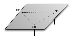
The table can be imagined as an infinite plane, defined by the points S0, S1, and S2. What we need to do is find the relation between velocities of S0, S1, and S2 such that an arbitrary point on the plane coincides with the center of rotation. Since this arbitrary point is a moving ball, we need to use dynamics equations for moving coordinate frames.
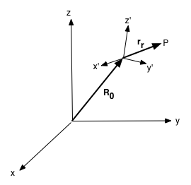
where R is the absolute xyz velocity of point P with respect to the origin; R0_dot=velocity of the origin of the moving reference frame, x'y'z'; rr_dot=velocity of point P relative to the x'y'z' system; and ω x r = cross product of the xyz angular velocity of the moving reference frame x'y'z' and the position vector rr. NOTE: because the coordinate systems are different, one cannot simply add together the values without first performing a transformation between the two systems.
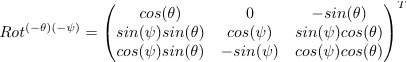
In order to convert the x'y'z' system into the xyz system, we need to define a rotation. Any orthogonal coordinate system can be brought to any other orthogonal coordinate by three successive rotations. However, in our case we will not rotate about the z axis, so we only need two rotations, one about the x-axis, and then a second about the new y-axis.
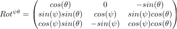
An important property of a rotation matrix is that its transpose is its inverse.
Next, it is useful to make several assumptions and definitions.
1) Since the ball is located on the plane at all time, the height above the plane, rrz, is identically 0, and thus are all its derivatives also.
2) Our moving coordinate axis is static about the z' -axis, i.e. ωz=0
3) The point P is constrained to move only along the z-axis. Moreover, this motion is our control, u.
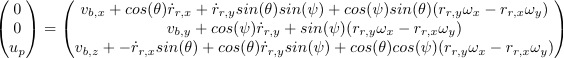
Applying the rotation matrix and the previous definitions to the original equation:
Now since we measure our state coordinates in the xyz frame, we must find the relation between the relative coordinates and the state ones. We can do this through a rotation.
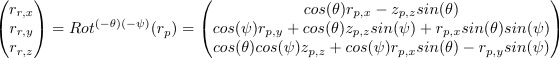
and equivalently:
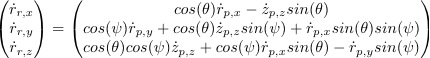
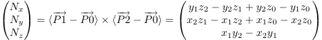
We can define
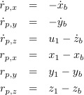
Also:

, where e is in the x'y'z' and N the xyz. Then
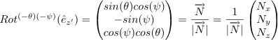
which allows us to solve for θ and ψ in terms of Nx, Ny, and Nz, which are NOT as previously defined because before the assumption was that z0 was stationary.
Substituting the above equations, we now have a simultaneous system where ωx, ωy , rpx_dot, and rpy_dot, are unknown. However, we only have three equations, which is insufficient for for unknowns.
Fortunately, we can get additional equations by considering other points on the plane. In this case, we'll consider the second point where the second actuator meets the table. Knowing that the rotational velocities ωx and ωy are identical with respect to all points, we can add a second set of movement equations and arrive at six equations and six unknowns.
Solving these simultaneous equations give us ωx, ωy, rpx1_dot, rpy2_dot, , rpx2_dot, and rpy2_dot in terms of only known constants.
Once we have these values, we can use them in a third point equation, this time corresponding to the third actuator, and obtain a value for u0.
ui can be seen as the relative speed of each actuator with respect to the plane. As we will see later, it will be necessary to add a uniform constant to the speed of each actuator in order to keep the table surface near the 0 point in order to have maximum control deflection. We'll deal more with this later.
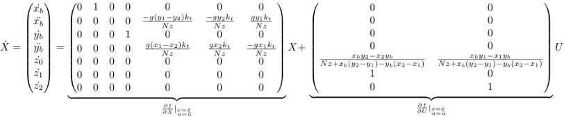
This yields the following a state-space system in the x_dot=Ax+f(x)+B(x,u) form:
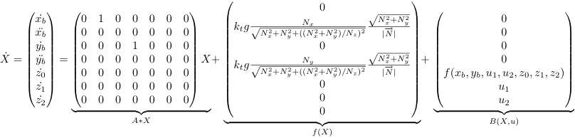
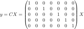
Also, let's add the output matrix:
This system is highly nonlinear, so a best first guess is to linearize about the equilibrium point (z0=0, z1=0, z2=0, u1=0, u2=0) by using the Jacobian.